Feature guides
Design Studio
The Design Studio is the flagship feature of the DataFlow AI Platform — a visual, node-based editor where you build ETL/ELT pipelines for Polkomtel's data estate. Its defining capability is tri-modal editing: the same pipeline can be edited as a visual DAG, as SQL, or as Python, and all three modes stay synchronized through one canonical YAML pipeline definition.
New here? Start with the plain-language picture
If you have never built a data pipeline before, do not worry — this section explains everything from scratch.
What is a pipeline? A pipeline is an automated recipe for moving data. It takes data out of one place (say, a sales database), tidies it up, and puts the finished result somewhere useful (say, a reporting warehouse). Once you write the recipe, the platform runs it for you — every night, every hour, or on demand — without anyone having to watch it.
What is ETL? ETL stands for Extract, Transform, Load — the three things a pipeline does:
- Extract — copy the raw data out of a source system.
- Transform — clean it, reshape it, and combine it (drop bad rows, fix formats, join tables together, hide private details).
- Load — write the finished data into a destination warehouse where analysts and dashboards can use it.
What is a node? A node is one box on the screen that does one job. A source node reads data in; a transform node changes it; a target (also called sink) node writes it out. You build a pipeline by dragging these boxes onto a canvas and drawing arrows between them.
What is a DAG? When you wire nodes together with arrows, you draw a DAG — a Directed Acyclic Graph. "Directed" means the arrows point one way (data flows forward, never backward). "Acyclic" means the arrows never loop back on themselves. In everyday terms: a DAG is a flowchart for your data, and the platform will refuse to run one that loops in a circle.
Think of the whole thing as an assembly line: data enters on the left, passes through stations that each do one task, and a finished product comes out on the right.
You do not have to write code
The Design Studio is drag-and-drop. You can build a complete, production-ready pipeline without typing a single line of SQL or Python. The SQL and Python modes exist for engineers who prefer code — but they are optional. A Business Analyst can build everything visually, or simply describe what they want to the AI Copilot and let it draft the pipeline.
What the Design Studio does
The Design Studio lets you compose a pipeline as a directed acyclic graph (DAG) of nodes — sources, transforms, quality checks, and targets — wired together by edges that carry data. Whatever you build is persisted as a Git-native YAML definition, so every action is versionable. ("YAML" is just a plain-text file format that records what your pipeline contains — you rarely need to look at it, but it is what makes every change trackable and reversible.)
Three editing modes operate on that single YAML:
- Visual — a React Flow (xyflow) drag-and-drop canvas.
- SQL — a Monaco editor showing the pipeline as chained CTEs.
- Python — a Monaco editor showing the pipeline as DataFlow SDK code.
Edit in any mode and the YAML updates; the other two modes re-derive their representation from it.
Routes: /design-studio (new pipeline), /design-studio?pipeline={id} (edit), /design-studio?template={id} (instantiate from a template). Entry file: src/pages/DesignStudio.tsx.
Who uses it
| Persona | How they use it |
|---|---|
| Data Engineer | Full power — drag-and-drop DAG building, SQL/Python modes, deploy controls |
| Business Analyst | Guided, AI-assisted building — often from a template or via the AI Copilot |
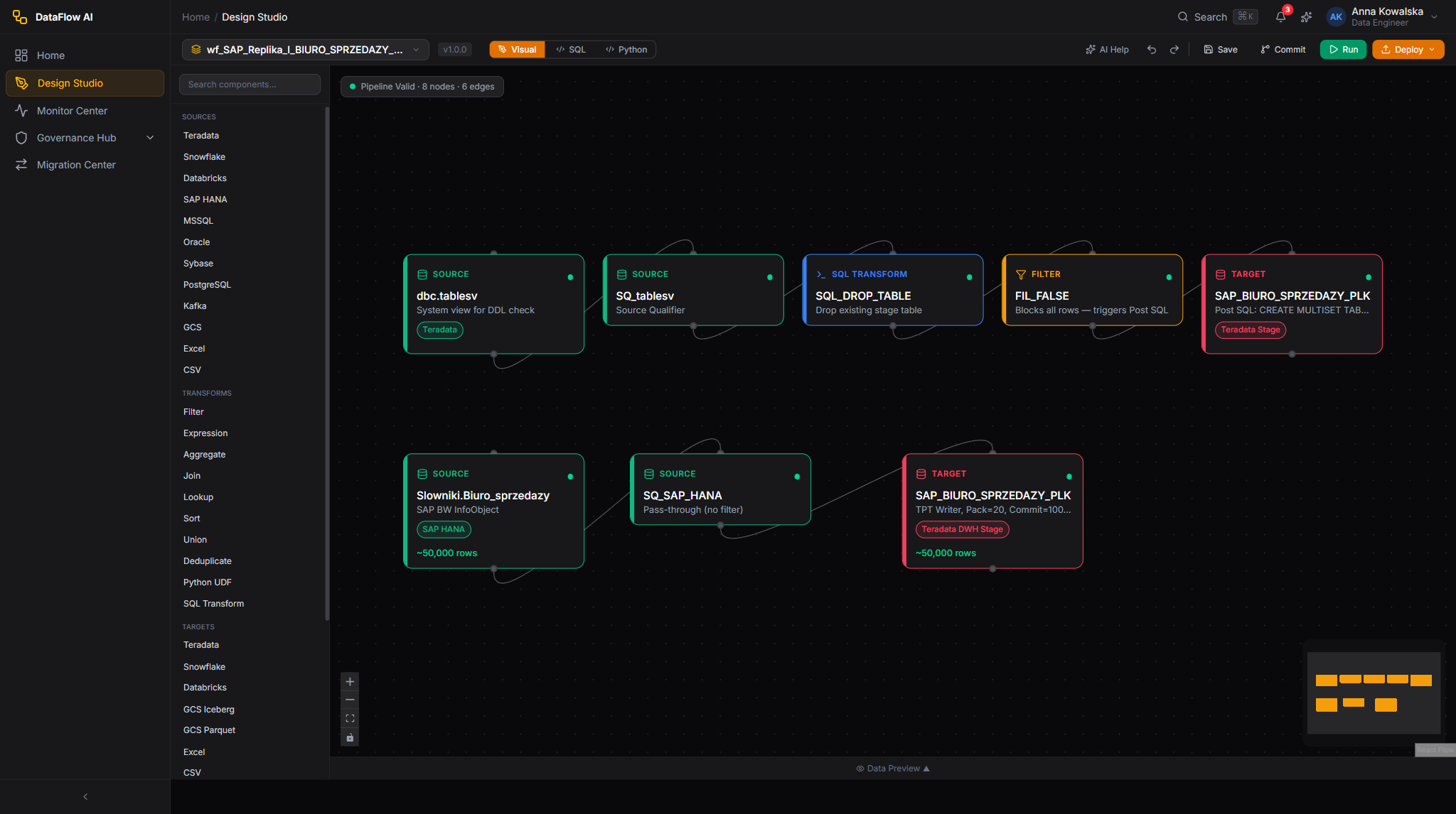
Screen layout
The Design Studio is a four-panel workspace. Every panel is resizable by dragging its divider, and panel sizes persist to localStorage under dataflow:studio:panels.
+==========================================================================+
| TOP TOOLBAR  [<] | Visual SQL Python | wf_SAP_Replika* | Validate Run Deploy|
+==========+===============================================+===============+
|          |                                               |               |
| LEFT     |              CENTER CANVAS                    |  RIGHT PANEL  |
| PANEL    |                                               |               |
|          |   React Flow DAG  (Visual mode)               |  Properties   |
| Component|        -- or --                               |  Inspector    |
| Palette  |   Monaco editor   (SQL / Python mode)          |  (selected    |
|          |                                               |   node config)|
| 240px    |              flex-1                           |   320px       |
+----------+-----------------------------------------------+---------------+
| BOTTOM PANEL   [Data Preview] [Console] [Test Results]   (collapsible)    |
+==========================================================================+
| Panel | Default size | Toggle |
|---|---|---|
| Left — Component Palette | 240px (200–400) | Ctrl+B |
| Right — Properties Inspector | 320px (280–500) | Ctrl+Shift+B |
| Bottom — Preview / Console | 240px (120–480) | Ctrl+J |
| Center — Canvas / Editor | flex-1 | — |
Double-clicking a divider resets that panel to its default size.
The Top Toolbar
The toolbar is split into three sections.
+==========================================================================+
| [<] Back | [Visual][SQL][Python] | wf_SAP_Replika_l_BIURO... [*] [pencil] |
| [Undo][Redo][Zoom-][Zoom+][Fit]  | [Validate]  [Run v]  [Deploy v]  [...] |
+==========================================================================+
| Control | What it does |
|---|---|
Back [<] | Returns to the /pipelines list |
| Mode toggle | Switches between Visual / SQL / Python |
| Pipeline name | Inline-editable; a * marks unsaved changes; a status badge shows draft/active/paused/error |
| Undo / Redo | Steps through edit history (Ctrl+Z / Ctrl+Shift+Z) |
| Zoom −/+ / Fit View | Canvas zoom controls |
| Validate | Runs pipeline validation; results land in the bottom Test Results tab |
| Run (split button) | Run / Run from selected node / Run with parameters / Dry run |
| Deploy (split button) | Deploy to Dev / Staging / Prod |
... menu | Save, Save As, Commit to Git, Export/Import YAML, Pipeline Settings, Delete |
The Component Palette (left panel)
The palette is a searchable node library (Ctrl+K focuses the search box) organized into five collapsible categories. Each entry shows an icon, label, short description, and a category color.
| Category | Count | Examples |
|---|---|---|
| Sources | 14 | Teradata, Snowflake, Databricks, SAP HANA, MSSQL, Oracle, Sybase, PostgreSQL, Kafka, GCS, Excel, CSV, JSON, XML |
| Transforms | 12 | Filter, Expression, Aggregate, Join, Lookup, Sort, Union, Deduplicate, Pivot, Unpivot, Python UDF, SQL Transform |
| Targets | 14 | Same connector set as Sources — bidirectional |
| Quality | 5 | Schema Validation, Null Check, Range Check, Format Check, Custom Rule |
| AI | 3 | AI Transform, AI Mapping, AI Suggestion |
Search filters by label, description, and category name. There is an AI button next to the search box that opens the AI Copilot with the context "Add a component to my pipeline." Each palette item can be dragged onto the canvas or double-clicked to auto-place it downstream of the last selected node.
What each transform node does — in plain words
Transform nodes are the "stations" on your assembly line. Here is what each one is for, with an everyday example.
| Transform | What it does | Real example |
|---|---|---|
| Filter | Keeps only the rows that match a condition; drops the rest | Keep only customers where STATUS = 'ACTIVE', throw away test accounts |
| Expression | Calculates or reformats columns, one row at a time | Add a LOAD_DATE column set to today's date; convert a phone number to a standard format |
| Aggregate | Summarizes many rows into fewer rows (a "GROUP BY") | Turn millions of call records into one total-minutes figure per region |
| Join | Combines two datasets into one by matching a shared key | Match each customer to their billing records using the customer ID |
| Lookup | Enriches each row by looking up an extra value from another table | Add a region name to each sale by looking up the store's postcode |
| Sort | Re-orders rows by one or more columns | Sort orders newest-first by order date |
| Union | Stacks rows from several datasets on top of each other | Combine this year's and last year's sales into one table |
| Deduplicate | Removes duplicate rows so each appears only once | Drop the same customer entered twice |
| Pivot / Unpivot | Rotates a table — turns rows into columns or columns into rows | Turn 12 monthly-total rows into one row with 12 month columns |
| Python UDF | Runs your own Python code for logic the built-in nodes cannot express | Run a machine-learning churn-score model on each customer |
| SQL Transform | Runs a hand-written SQL statement against upstream data | A complex multi-table calculation you would rather express in SQL |
Quality nodes (Schema Validation, Null Check, Range Check, Format Check, Custom Rule) do not change data — they inspect it and raise a flag if something is wrong. Placing one right after a source node is a good habit: it catches bad data before it spreads through the rest of your pipeline.
The canvas (Visual mode)
The center canvas is a React Flow DAG editor.
| Feature | Detail |
|---|---|
| Pan | Drag empty canvas |
| Zoom | Scroll wheel or Ctrl+= / Ctrl+-, range 25%–200% |
| Multi-select | Shift+click or rubber-band selection |
| Snap to grid | 20px grid, toggle via toolbar |
| Minimap | Bottom-right corner |
| Auto-layout | Dagre top-to-bottom layout |
| Context menus | Right-click on canvas or on a node |
Node design system
Nodes are 220px wide and color-coded by category:
| Category | Color | Badge |
|---|---|---|
| Sources | Blue | SRC |
| Transforms | Violet | TRF |
| Targets | Orange | TGT |
| Quality | Emerald | QA |
| AI | Amber | AI |
Each node carries an 8px status dot (top-left), a category badge (top-right), and a row-count badge (bottom). Node states: idle, selected (3px border + glow ring), hover, running (pulsing border), success (green check), error (red border + glow), and disabled (50% opacity with a striped overlay).
Ports are 12px circles — inputs on the top edge, outputs on the bottom edge. While you drag a connection, valid target ports turn blue and scale up; invalid ports turn red.
Edges use the smoothstep style, animate during runs, and display a row-count pill at their midpoint. Hovering an edge shows a delete X.

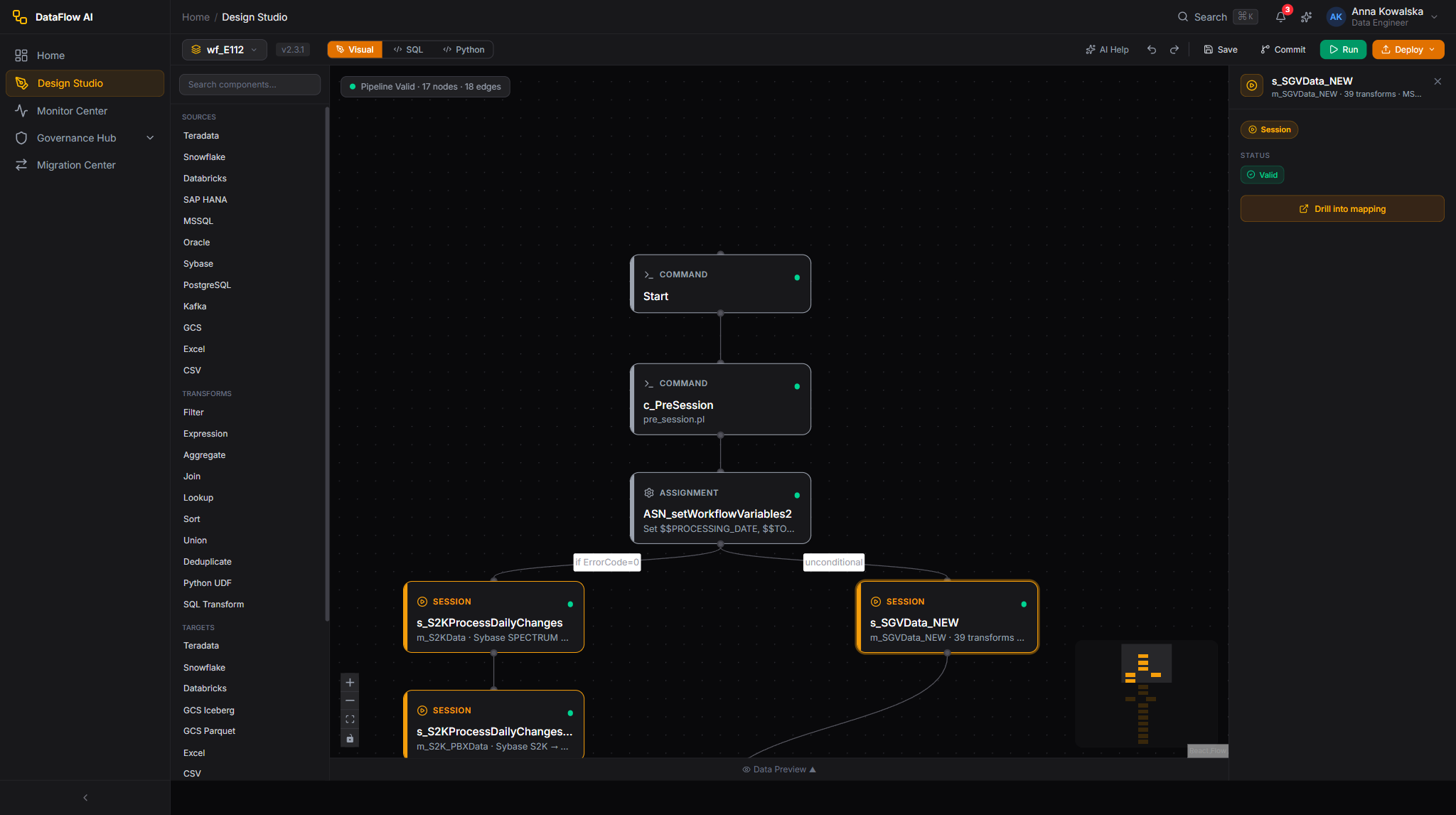
The Properties Inspector (right panel)
When a node is selected the right panel shows four tabs.
| Tab | Contents |
|---|---|
| General | Type-specific configuration fields (connection, schema, table, write mode, etc.) |
| Schema | The node's output columns table, with Infer Schema / Edit Schema / add-column controls |
| Preview | A compact 20-row data preview of the node's output |
| Advanced | Node ID, execution engine, parallelism, timeout, retry count/delay, error handling, custom properties, tags, notes |
For example, a SAP HANA source General tab includes Display Name, Connection, Schema, Table/View, optional Custom SQL, Extract Mode (full / incremental / cdc), Watermark Column, and Fetch Size. A Teradata target adds Write Mode (insert / upsert / merge / replace / append), Key Columns, Pre-SQL/Post-SQL, and Batch Size.
When no node is selected, the panel invites you to select a node or open Pipeline Settings.
The Bottom Panel
A collapsible panel (Ctrl+J) with three tabs:
| Tab | Contents |
|---|---|
| Data Preview | A virtualized TanStack Table of sample rows at the selected node |
| Console | A color-coded log stream — INFO gray, WARN amber, ERROR red, OK green |
| Test Results | A PASS/FAIL list per validation check, with a re-run control |
The SQL editor
Switching to SQL mode replaces the canvas with a Monaco editor. The pipeline is rendered as a series of chained CTEs:
-- Pipeline: wf_SAP_Replika_l_BIURO_SPRZEDAZY_PLK
-- Dialect: Teradata

WITH source_sap_hana AS (
    SELECT * FROM sap_hana_plk.BIURO_SPRZEDAZY
),
filtered AS (
    SELECT * FROM source_sap_hana WHERE STATUS = 'ACTIVE'
),
enriched AS (
    SELECT *,
           CURRENT_TIMESTAMP AS LOAD_DATE,
           'SAP_HANA_PLK' AS SOURCE_SYSTEM
    FROM filtered
)
INSERT INTO teradata_dwh_mona.STG_BIURO_SPRZEDAZY_PLK
SELECT * FROM enriched;
The SQL editor toolbar provides a Dialect dropdown (ANSI, Teradata, Snowflake, Databricks, PostgreSQL, MSSQL), plus Format, Validate, and Explain buttons. IntelliSense autocompletes tables, columns, and dialect-specific functions; the AI Copilot offers grey ghost-text suggestions that you accept with Tab.
The Python editor
Switching to Python mode shows the pipeline as DataFlow SDK code:
from dataflow import Pipeline
from dataflow.connectors import SAPHana, Teradata
from dataflow.transforms import Filter, Expression

pipeline = Pipeline(name="wf_SAP_Replika_l_BIURO_SPRZEDAZY_PLK",
                    schedule="0 */2 * * *")

source = pipeline.add_source(
    SAPHana(connection="sap_hana_plk", schema="BIURO_SPRZEDAZY",
            mode="incremental", watermark_column="LAST_MODIFIED"))

filtered = source.pipe(Filter(condition="STATUS = 'ACTIVE'"))
enriched = filtered.pipe(Expression(columns={
    "LOAD_DATE": "CURRENT_TIMESTAMP",
    "SOURCE_SYSTEM": "'SAP_HANA_PLK'"}))

enriched.write_to(Teradata(connection="teradata_dwh_mona",
                           table="STG_BIURO_SPRZEDAZY_PLK",
                           mode="merge", keys=["ID"], push_down=True))
The Python editor toolbar offers Format (Black rules), Lint, and Run Cell, plus DataFlow SDK autocomplete and AI ghost-text suggestions.
Walkthrough — build your very first pipeline, step by step
This is a complete, beginner-friendly walkthrough. The goal: build a pipeline that copies sales data from SAP HANA into a Teradata warehouse, dropping test rows and stamping each row with the load date. Follow it click by click — it takes about ten minutes.
Before you start: confirm a workspace administrator has already registered the connections you need (here, a SAP HANA source connection and a Teradata target connection). A connection is a saved, reusable login to an external system. If a connection is missing, ask your administrator — you cannot create connections from the Design Studio.
- Open the Design Studio. On the Home Dashboard, click New Pipeline in the Quick Actions bar. A blank canvas opens.
- Name the pipeline. Click the pipeline name in the top toolbar (it starts as "Untitled") and type a clear name, for example
wf_Sales_Daily_Load. Clear names make later troubleshooting far easier. - Add the source. In the left Component Palette, open the Sources category, find SAP HANA, and drag it onto the canvas. A blue box appears.
- Configure the source. With the SAP HANA node selected, look at the right Properties Inspector → General tab. Pick your Connection from the dropdown, choose the Schema and Table (for example
BIURO_SPRZEDAZY), and set Extract Mode toincrementalso the pipeline only pulls new rows each run rather than re-reading everything. - Add a Filter. From the palette's Transforms category, drag a Filter node onto the canvas, to the right of the source.
- Connect the source to the filter. Hover the bottom edge of the SAP HANA node until a small circle (the output port) appears. Click and drag from that circle to the input port on the top edge of the Filter node. An arrow snaps into place — data now flows from source to filter.
- Configure the Filter. Select the Filter node and, in the General tab, type the condition
STATUS = 'ACTIVE'. This keeps live sales and discards test rows. - Add an Expression. Drag an Expression node to the right of the Filter and connect Filter → Expression the same way. In its General tab, add a new column named
LOAD_DATEwith the valueCURRENT_TIMESTAMP. Every row will now carry the moment it was loaded. - Add the target. From the Targets category, drag a Teradata node onto the canvas and connect Expression → Teradata.
- Configure the target. Select the Teradata node. Pick the Connection, set the destination Table, and choose a Write Mode — pick
upsertfor a daily load (it updates rows that already exist and inserts the new ones). Set the Key Columns (for exampleID) so the platform knows how to match existing rows. - Validate. Click Validate in the toolbar. The bottom Test Results tab lists any problems — a missing required field, a disconnected node, or a schema mismatch. Fix anything flagged in red.
- Preview the data. Right-click any node and choose Preview Data to see up to 20 sample rows at that point in the pipeline. This is the quickest way to confirm a Filter or Expression is doing what you expect.
- Run it once. Click Run. An execution overlay appears, the nodes animate, and the Console tab streams live log lines. Wait for every node to turn green.
- Schedule it. Open the
...menu → Pipeline Settings and set a schedule, for example0 2 * * *(every day at 2 AM). See the cron table in the FAQ below if cron expressions are new to you. - Deploy. Click Deploy and choose an environment — start with Dev, then promote to Staging and Prod once you trust it. The schedule only becomes active after the pipeline is deployed.
That's it — you have built, tested, scheduled, and deployed a working pipeline.
Auto-save has your back
The Design Studio auto-saves your work every 30 seconds, and your login session lasts 8 hours. You will not lose a half-built pipeline if your browser closes — but still click Save (Ctrl+S) before you walk away.
Click-paths
Build a pipeline visually
- Open the Design Studio (e.g. via New Pipeline on the Home Dashboard).
- From the left Component Palette, drag a source node — say Teradata — onto the canvas. (Or double-click it to auto-place.)
- Drag from the source node's bottom output port to a transform node's top input port to create an edge.
- Select each node and configure it in the right panel's General tab.
- Drag a Target node onto the canvas and connect the last transform to it.
- Click Validate in the toolbar — results appear in the bottom Test Results tab.
- Click Run — an execution overlay appears, node statuses animate, and the Console tab streams logs.
- When the run succeeds, click Deploy → Deploy to Staging.
Write a SQL pipeline
- In the toolbar, click SQL in the mode toggle — the canvas becomes a Monaco editor.
- Choose your target Dialect (e.g. Teradata) from the dropdown.
- Write or edit the chained-CTE SQL; accept AI ghost-text suggestions with
Tab. - Click Format to normalize the SQL, then Validate to check syntax against the target systems.
- Optionally click Explain to view the estimated execution plan.
- Switch back to Visual mode at any time — the DAG re-derives from your SQL.
Schedule a pipeline
- With your pipeline open, click the
...menu in the toolbar. - Choose Pipeline Settings.
- Set the schedule (a cron expression, e.g.
0 */2 * * *for every two hours). - Save the pipeline (
Ctrl+Sor...→ Save). - Click Deploy and pick the target environment — the schedule becomes active once the pipeline is deployed.
Inspect data at a node
- Right-click any node on the canvas.
- Choose Preview Data.
- The bottom panel opens to the Data Preview tab with sample rows and profiling for that node.
Instantiate a pipeline from a template
- Open the Pipeline Templates gallery and click Use Template on a card.
- You arrive at
/design-studio?template={id}with the Studio pre-populated by that template. - Adjust connections and configuration, then Validate, Run, and Deploy.
The three modes never diverge
Because Visual, SQL, and Python all derive from one canonical YAML definition, you can move fluidly between them. A change in any mode updates the YAML; the other modes re-render from it the next time you switch.
Tips and best practices
A few habits make pipelines reliable, cheap, and easy to debug.
- One pipeline, one job. Keep each pipeline focused on a single logical task. Avoid "mega-pipelines" with 50+ nodes — split the work into smaller pipelines that hand off through staging tables. The canvas stays smooth up to about 100 nodes, but smaller is easier to reason about.
- Always load incrementally. Set source nodes to
incrementalmode and add a date filter so each run pulls only new rows. Re-scanning a huge table every night is slow and expensive. - Add a quality gate early. Place a Quality node (such as a Null Check) right after the source. Catching bad data at the door stops it polluting everything downstream.
- Name nodes clearly.
src_sap_crm_customerstells you far more in a log file thansource1. Good names also make the AI Copilot's diagnostics sharper. - Never hardcode values. Use pipeline parameters for dates, table names, and environment differences instead of typing them into expressions.
- Set a realistic timeout. In Pipeline Settings, set the timeout to roughly twice the expected run time, so a genuinely stuck run is auto-cancelled but a normal slow night is not.
- Test before you schedule. Run the pipeline manually at least once and check the output row count and a sample of the target table before turning on the cron schedule.
- Validate before you deploy. Treat the Validate button as mandatory — and a Dry run as a good idea — before promoting to Staging or Prod.
Common questions
Do I need to know SQL to use the Design Studio? No. The visual drag-and-drop mode builds complete pipelines with no code. SQL and Python modes are optional conveniences for engineers who prefer them.
What does "tri-modal" mean? The same pipeline can be edited three ways — as a visual diagram, as SQL, or as Python — and all three always agree, because they are different views of one underlying definition. Edit in whichever mode suits the task; switch freely.
What is a "write mode" and which should I pick? The write mode tells the target how to add your data:
| Write mode | What it does | When to use it |
|---|---|---|
append / insert | Adds new rows alongside existing ones | Event logs where rows are never updated |
overwrite / replace | Deletes everything, then writes fresh | Small reference tables rebuilt each run |
upsert / merge | Updates rows that already exist, inserts new ones | The usual choice for daily warehouse loads |
How do I schedule a pipeline, and what is a cron expression? A cron expression is a five-field code that says "run on this schedule". Open Pipeline Settings → Schedule and enter one:
| Cron expression | Meaning |
|---|---|
0 2 * * * | Every day at 02:00 |
0 6 * * 1-5 | Weekdays at 06:00 |
0 0 1 * * | The 1st of every month at midnight |
0 */4 * * * | Every 4 hours |
30 8,20 * * * | At 08:30 and 20:30 every day |
The default timezone is Europe/Warsaw, and Polish public holidays can be set as exclusion days so a run skips them.
My pipeline saved but the Run button is greyed out — why? You can save a pipeline that still has validation errors, but you cannot run it until they are fixed. Click Validate and resolve every red marker in the Test Results tab.
Can two people edit the same pipeline at once? Yes — the canvas supports real-time collaborative editing, so you see each other's changes live.
How do I undo a mistake? Press Ctrl+Z (undo) or Ctrl+Shift+Z (redo). The Studio keeps a deep edit history. For older versions, use ... menu → version history to compare and restore.
Where does my pipeline go when I save it? Into a Git version-control repository as a YAML file. Every save is a tracked change, so you can always see what changed and roll back.
Behind the scenes
| Concern | API / module |
|---|---|
| Pipeline CRUD and run | api/pipelines.ts (PipelineDto) |
| AI assistance | api/textToSql.ts, api/copilot.ts |
| Schema inference & autocomplete | api/catalog.ts (metadata service) |
| Version control | api/git.ts — YAML is the persisted canonical form |
Validate before you deploy
The Deploy button promotes a pipeline to a real environment. Always run Validate (and ideally a Dry run) first so connection, schema, and quality-rule errors surface in the Test Results tab before they reach Staging or Prod.